Thomas Denecker & Claire Toffano-Nioche


Session 7
21/06/2019
Novembre
Janvier
Février
Mars
Avril
Mai
Juin
Juillet
...
26
25
22
29
26
24
21
...
5
Session 7
Les notebooks
C'est quoi un notebook?
Interface de programmation interactive permettant de combiner des sections en langage naturel et des sections en langage informatique.
Pourquoi un notebook ?
Rapport d'analyse
Simple à exporter
Rendre toutes les informations de l'analyse disponibles
(code + résultats + graphiques)
Disponible pour de très nombreux langages
(R, Python, ...)
Programme de la session
Markdown
Jupyter / Jupyterlab
- Docker Jupyter
- Mise en ligne avec Binder
Rmarkdown
Générer le notebook de l'application shiny
Markdown

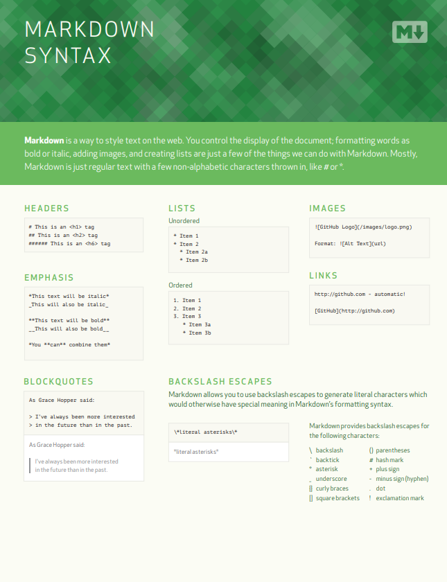
Markdown
Langage simple de balises
Vous connaissez déjà !
C'est le langage utilisé dans le README de Github!
Github guides : https://guides.github.com/features/mastering-markdown/
Rappel
Une page de wiki est disponible sur FAIR_bioinfo
https://github.com/thomasdenecker/FAIR_Bioinfo/wiki/Markdown
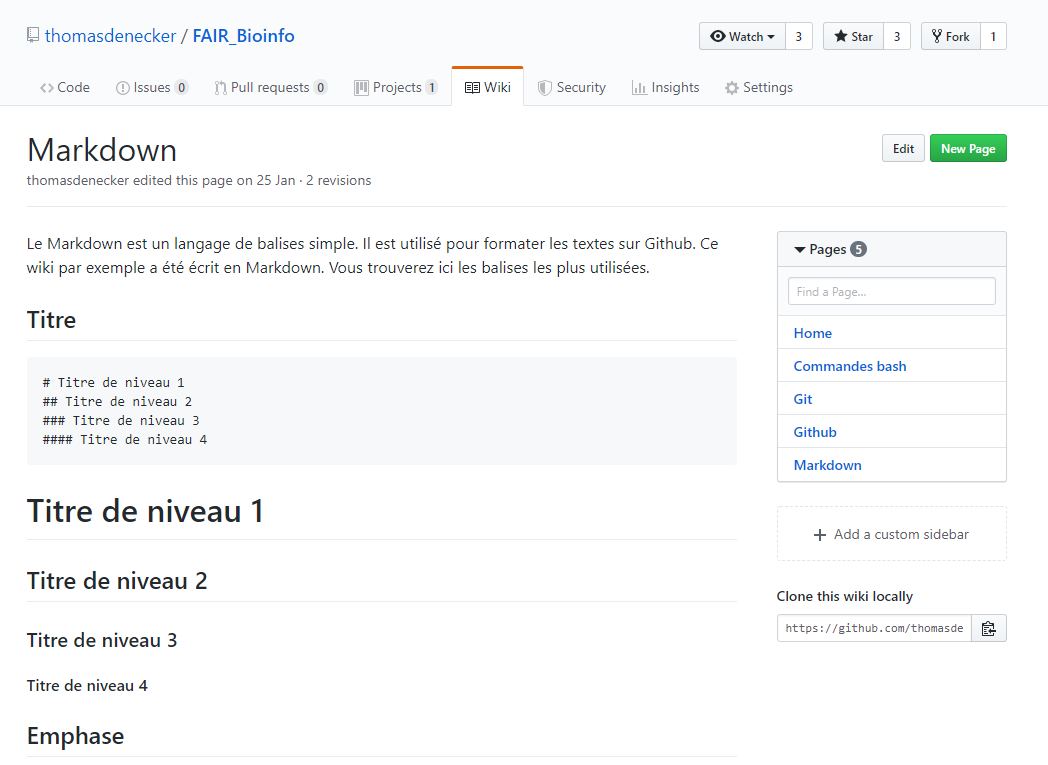
Revue rapide des commandes de base
- Titre
- Emphase
- Liste
- Image
- Lien
- Citation
- Liste de tâches
- Tableau
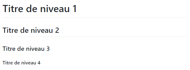
Titre
Code
# Titre de niveau 1
## Titre de niveau 2
### Titre de niveau 3
#### Titre de niveau 4
Rendu
Italique
Code
*Un texte en italique*
_Un texte aussi en italique_
Rendu

Gras
Code
**Un texte en gras**
__Un texte aussi en gras__
Rendu

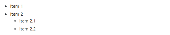
Liste désordonnée
Code
* Item 1
* Item 2
  * Item 2.1
  * Item 2.2
Rendu
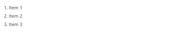
Liste ordonnée
Code
1. Item 1
2. Item 2
3. Item 3
Rendu
Image
Code
Rendu
L'adresse peut être locale (adresse relative) ou une URL

Lien
Code
[Github](https://github.com/)Rendu

Citation
Code
Mireille Sitbon a dit :
> L'informatique, ça fait gagner beaucoup de temps...
> à condition d'en avoir beaucoup devant soi !
Rendu

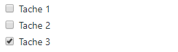
Liste de tâches
Code
- [ ] Tache 1
- [ ] Tache 2
- [x] Tache 3
Rendu
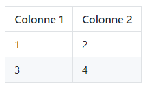
Tableau
Code
Colonne 1 | Colonne 2
----------|----------
1         |2
3         |4
Rendu
Markdown a aussi sa cheat sheet

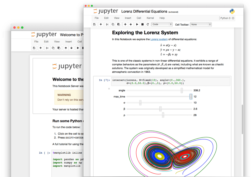
Jupyter Project
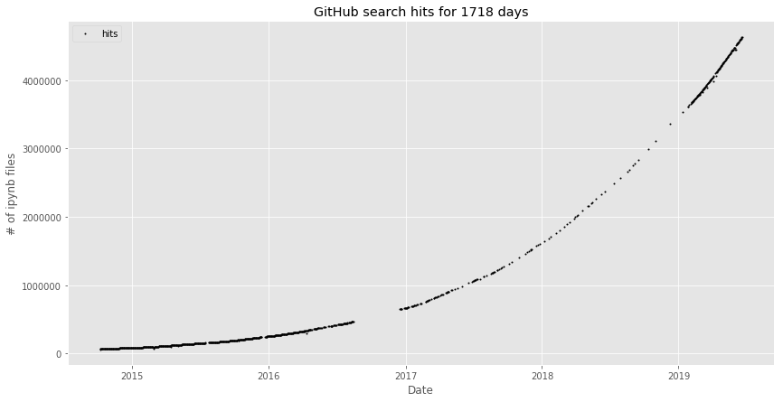
Un project en plein essor !
https://nbviewer.jupyter.org/github/parente/nbestimate/blob/master/estimate.ipynb
Environ 4.6 millions de notebook jupyter sur Github !
(20/06/2019)
Jupyter est utilisé par les plus grands


...
De nombreux articles en parlent
This year’s Nobel Prize in economics was awarded to a Python convert, Kopf , 2018
Jupyter: Tools for the Life Cycle of a Computational Idea, Siam News, 2018
Interactive notebooks: Sharing the code, Shen, Nature, 2014
By Jupyter it all makes sense, Perkel, Nature, 2018
Dans tous les domaines
Informatique
Statistiques
Psychologie
Social
Finances
Mathématiques
Chimie
Physique
...
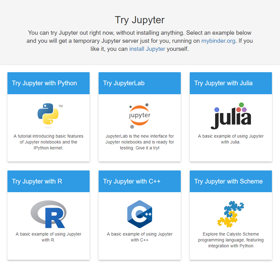
Des exemples
Tester en ligne
Différents notebooks sont disponibles pour tester (modifiables et rejouables)
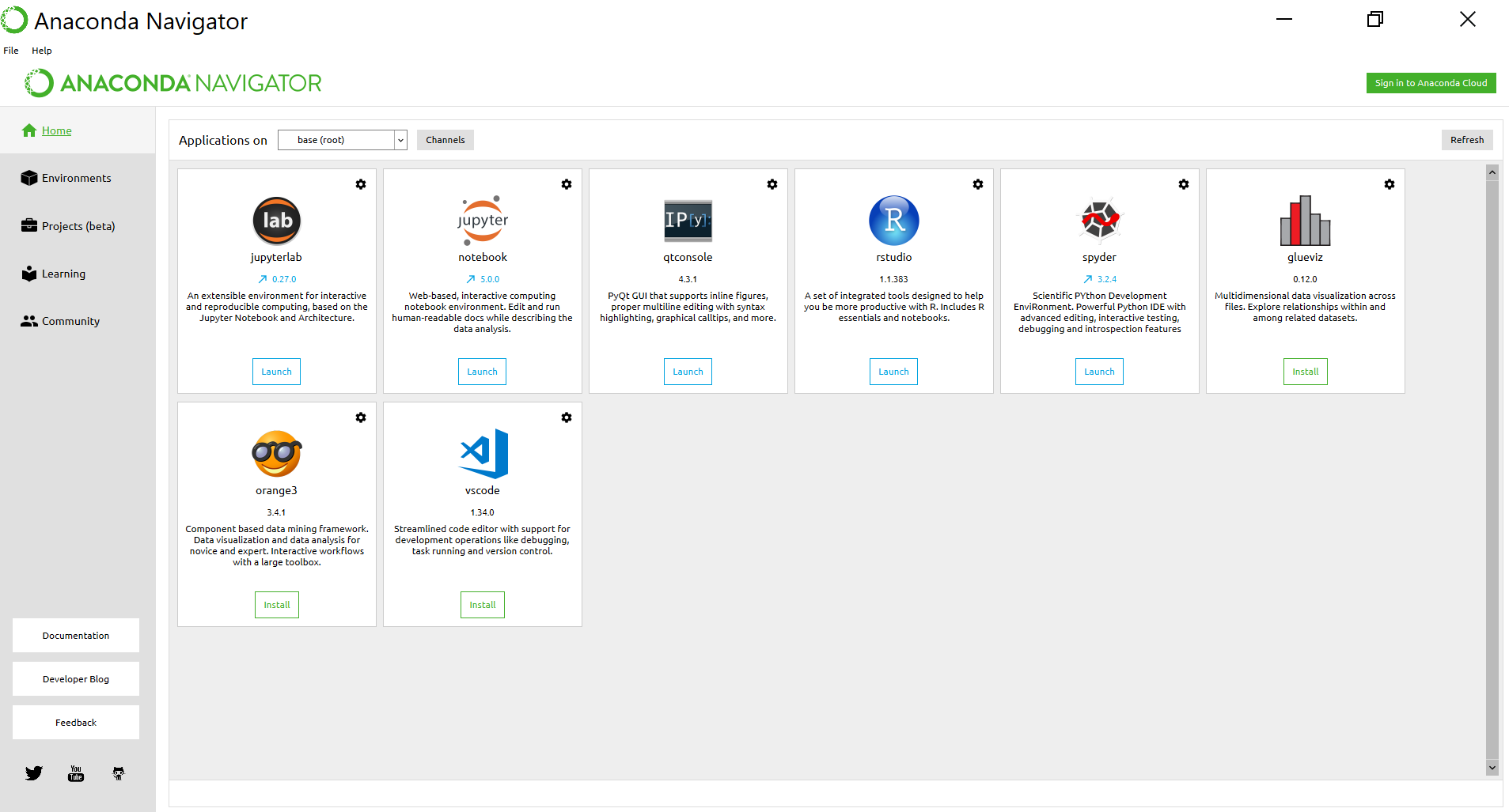
Installation par Anaconda
Déjà installé par défaut
Méthode la plus simple (la moins reproductible ? )
Installation (terminal)
python3 -m pip install --upgrade pip
python3 -m pip install jupyter
Pip install
conda install -c anaconda jupyter Conda
Pour le lancer
jupyter notebookDocker
Proposé par Jupyter
Nombreux kernel pré-installés
docker run --rm -p 8888:8888 -p 4040:4040 -v ${PWD}:/home/jovyan/work jupyter/all-spark-notebookPuis
Copier l'adresse du message dans un navigateur
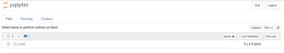
Dans le dossier work se trouve votre dossier partagé
(-v, volume)
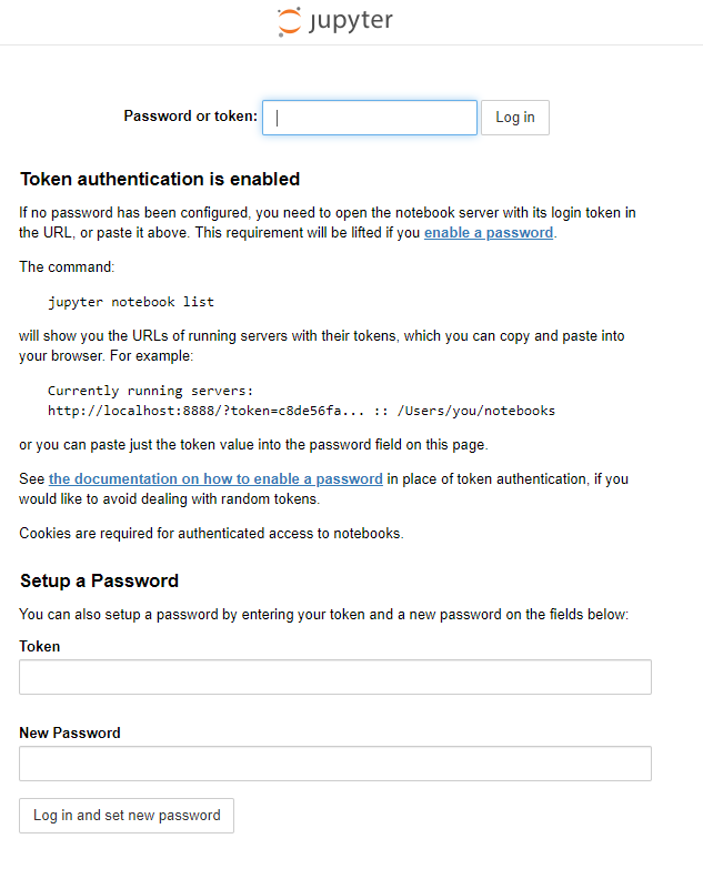
Ouvrir un notebook Jupyter avec Docker Solution 1
Executing the command: jupyter notebook
[I 08:31:13.762 NotebookApp] Writing notebook server cookie secret to /home/jovyan/.local/share/jupyter/runtime/notebook_cookie_secret
[I 08:31:14.645 NotebookApp] JupyterLab extension loaded from /opt/conda/lib/python3.7/site-packages/jupyterlab
[I 08:31:14.645 NotebookApp] JupyterLab application directory is /opt/conda/share/jupyter/lab
[I 08:31:14.647 NotebookApp] Serving notebooks from local directory: /home/jovyan
[I 08:31:14.647 NotebookApp] The Jupyter Notebook is running at:
[I 08:31:14.648 NotebookApp] http://(716ae9fc149a or 127.0.0.1):8888/?token=2996432e3056fc62c38bd40d135824a5d586f59cc244c6f9
[I 08:31:14.648 NotebookApp] Use Control-C to stop this server and shut down all kernels (twice to skip confirmation).
[C 08:31:14.653 NotebookApp]

    To access the notebook, open this file in a browser:
        file:///home/jovyan/.local/share/jupyter/runtime/nbserver-6-open.html
    Or copy and paste one of these URLs:
        http://(716ae9fc149a or 127.0.0.1):8888/?token=2996432e3056fc62c38bd40d135824a5d586f59cc244c6f9
Utiliser plutôt 127.0.0.1 :
http://127.0.0.1:8888/?token=2996432e3056fc62c38bd40d135824a5d586f59cc244c6f9
Ouvrir un notebook Jupyter avec Docker Solution 2
Lancer http://localhost:8888
Copier la clé située après token=
http://127.0.0.1:8888/?token=2996432e3056fc62c38bd40d135824a5d586f59cc244c6f9
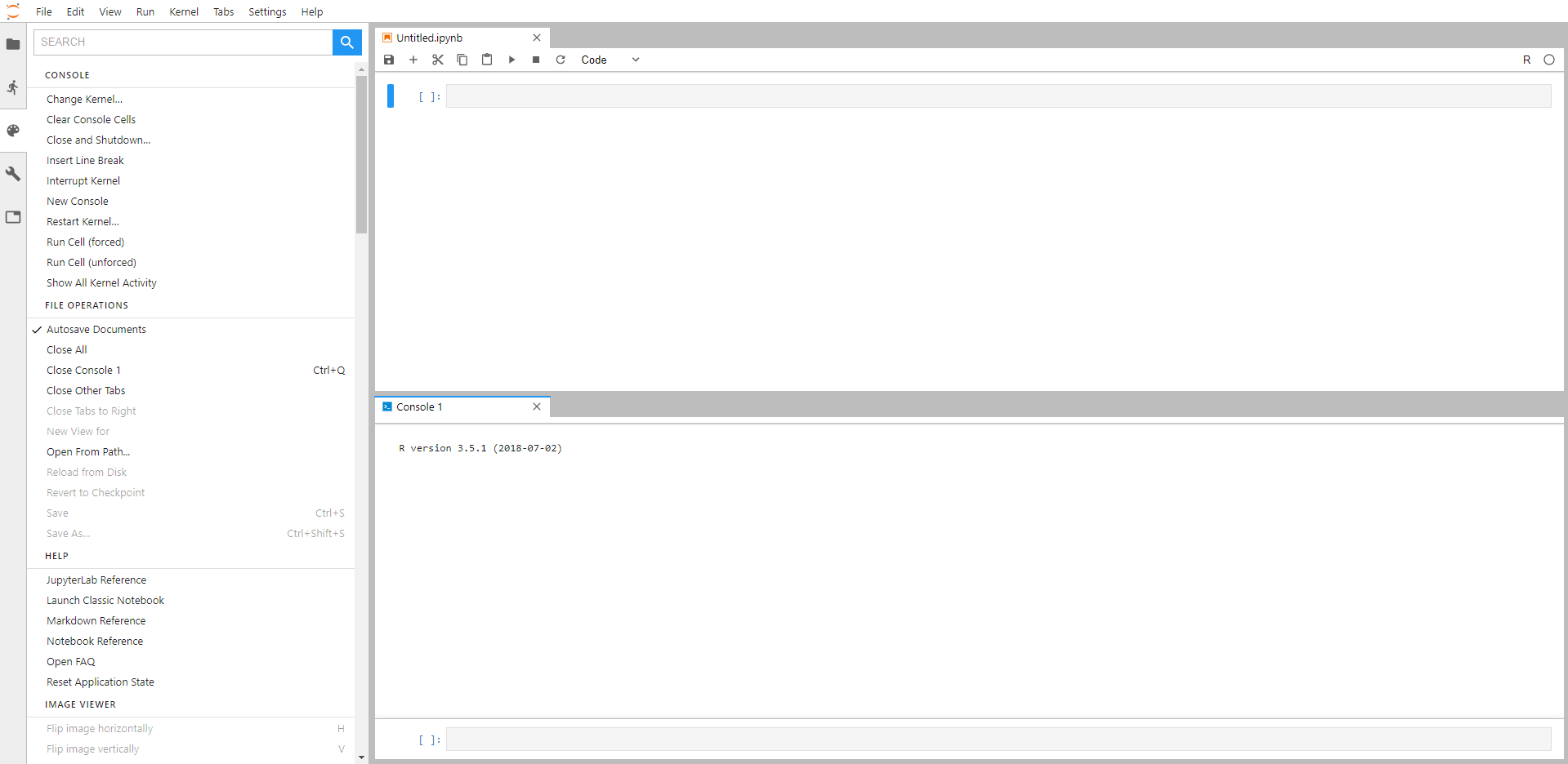
Création d'un notebook
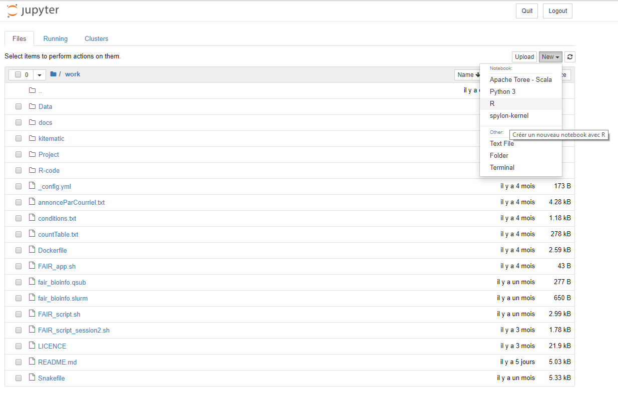
Dans le notebook
Kernel utilisé
Cellule
Type de cellule
(code ou markdown)
Exécuter la cellule
Avant exécution
Après exécution


Prendre le contrôle sur le notebook
Partager un Notebook Jupyter
Partage avec Github
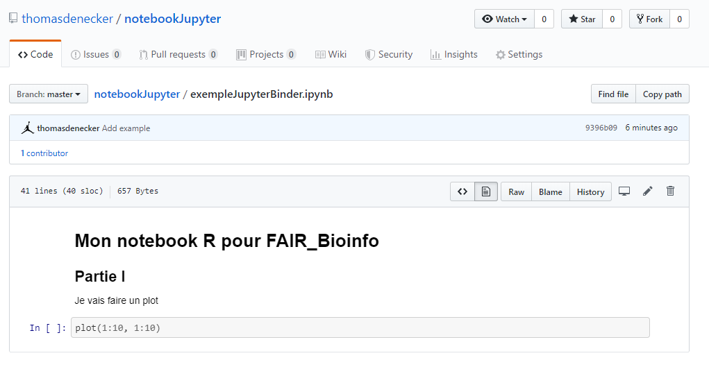
Rejouer mon notebook
A partir de Github avec Binder !
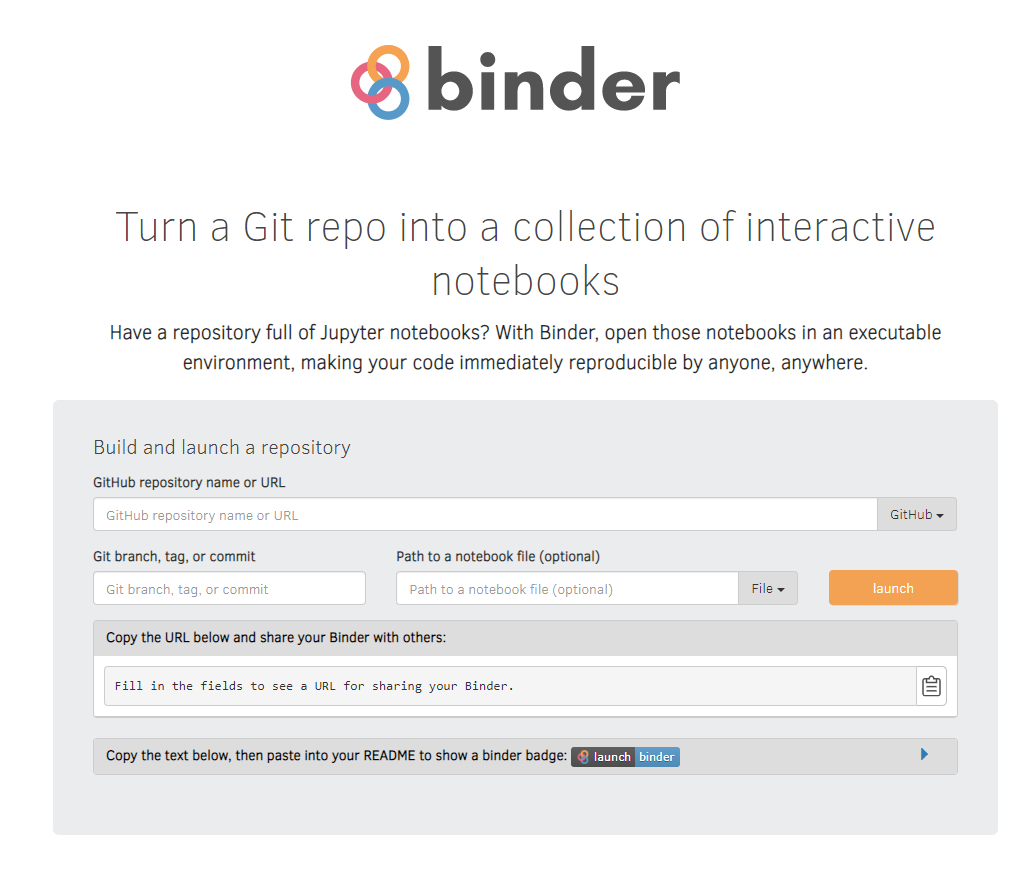
Création d'un lanceur pour votre README
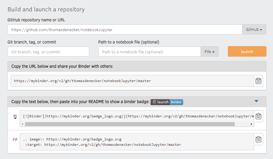
Il travaille avec Docker.
Il construit l'image avec le dockerfile présent dans le repo !
Le lancement peut être un peu long (téléchargement de l'environnement)


Le Dockerfile de l'exemple
FROM rocker/binder

## Copies your repo files into the Docker Container
USER root
COPY . ${HOME}
RUN chown -R ${NB_USER} ${HOME}

## Become normal user again
USER ${NB_USER}
Binder et le Dockerfile
Si nous mettons binder sur notre repo FAIR_bioinfo, il reconstruit l'image à partir du fichier Dockerfile
=> Pas reproductible
Nous utilisons par contre l'image disponible sur Dockerhub pour utiliser exactement la même
=> Reproductible
Attention !
Ici nous n'utilisons pas notre image car elle est trop lourde.
Une solution : faire plusieurs dockers (1 docker = 1 outil)
Notre notebook dans binder
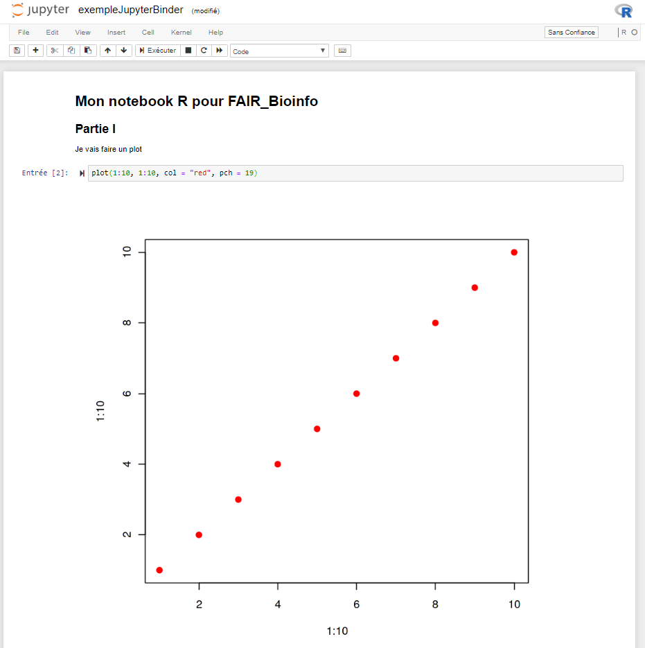
Possible de faire des modifications dans le notebook et de les exécuter
Interface identique
JupyterLab
IDE de Jupyter
Lancer JupyterLab
Docker
Même système pour se connecter que Jupyter
docker run --rm -p 8888:8888 -p 4040:4040 -e JUPYTER_ENABLE_LAB=yes -v ${PWD}:/home/jovyan/work jupyter/all-spark-notebookpython3 -m pip install jupyterlab
jupyter labConda
conda install -c conda-forge jupyterlab
jupyter lab
Pip
Dans JupyterLab
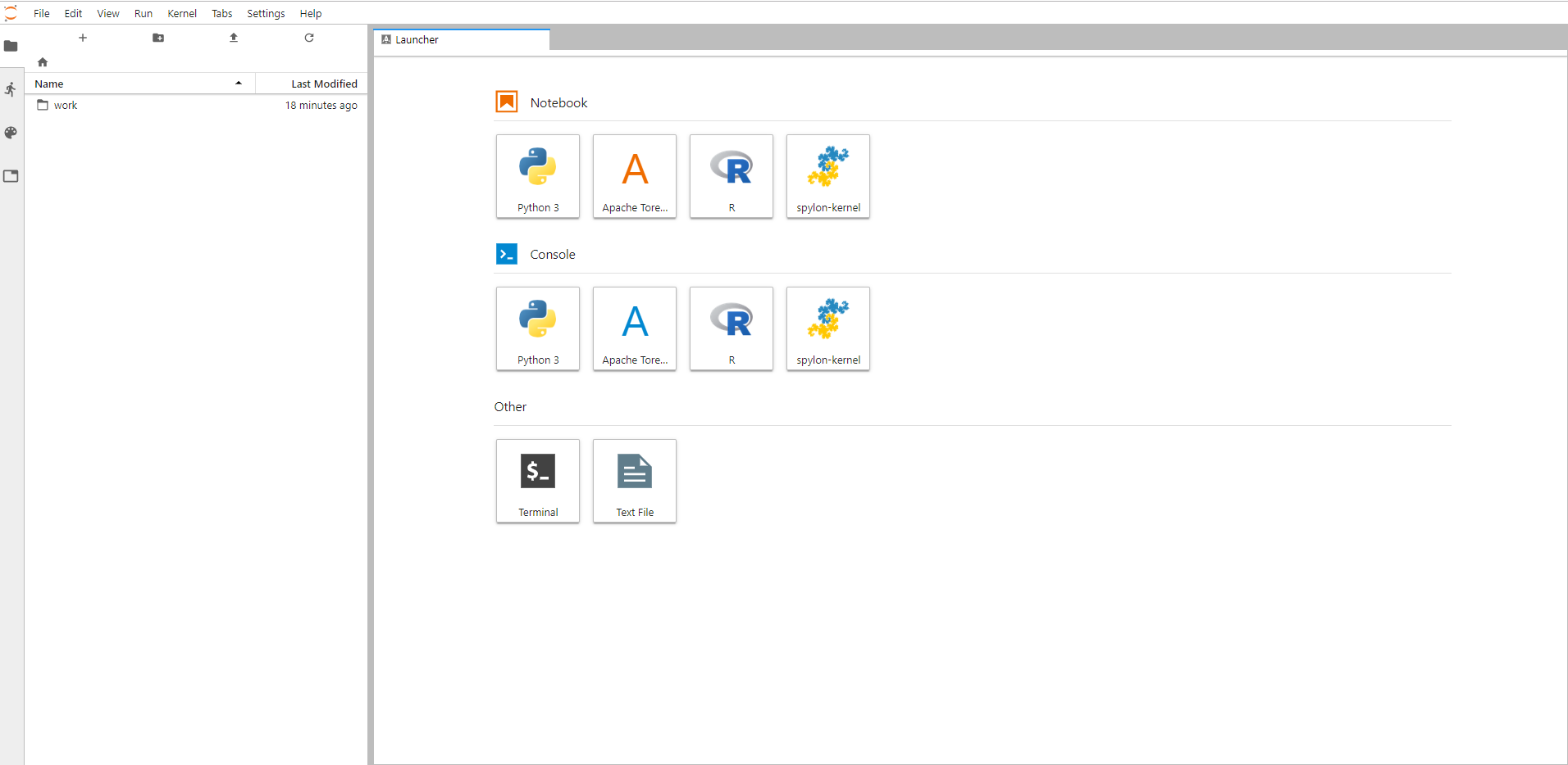
Création d'un notebook
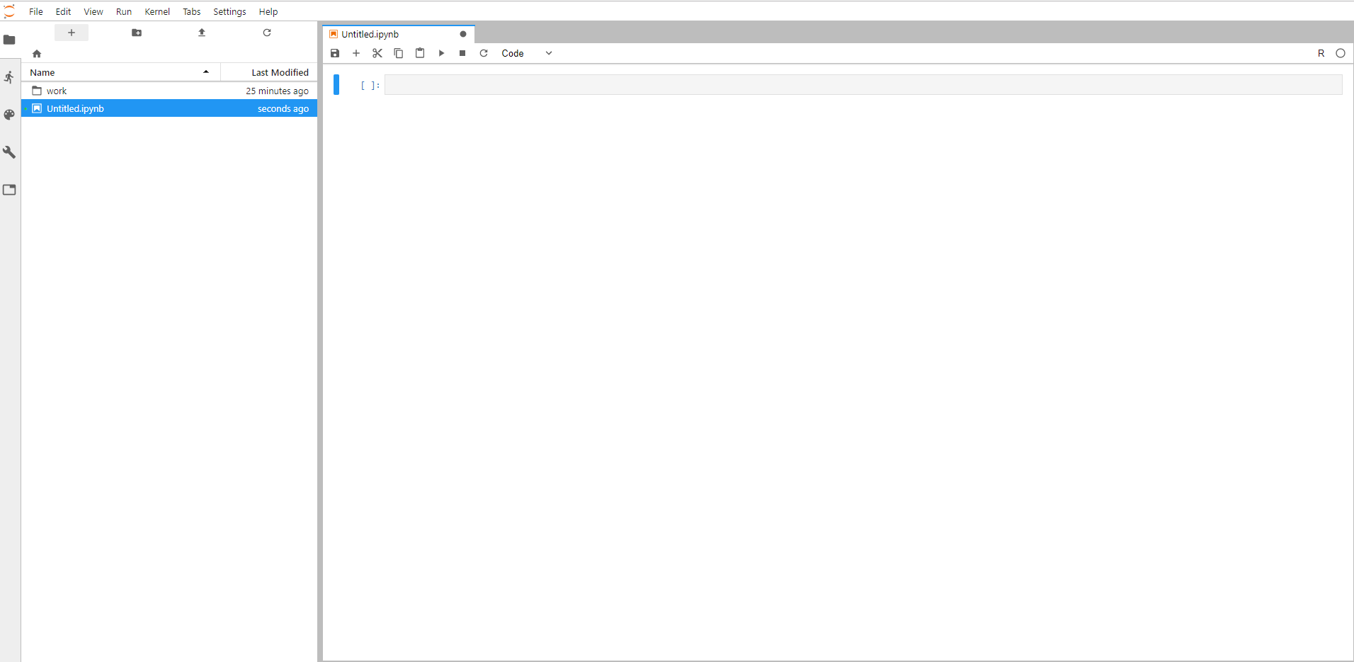
Mêmes principes que Jupyter
Pourquoi utiliser JupyterLab
Fenêtre paramétrable

Rmarkdown

+
Dans Rstudio
Avec notre docker
docker run --rm -d -p 80:8888 --name fair_bioinfo -v ${PWD}:/home/rstudio tdenecker/fair_bioinfoNote - Notre docker est une combinaison de Jupyter, Binder et Rstudio
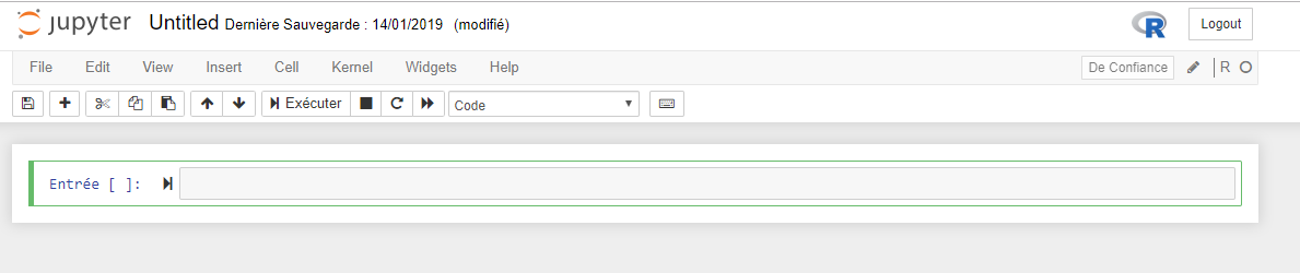
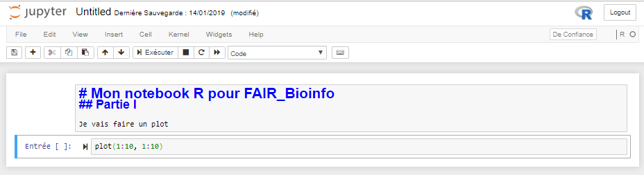
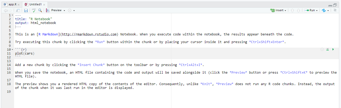
Création d'un notebook
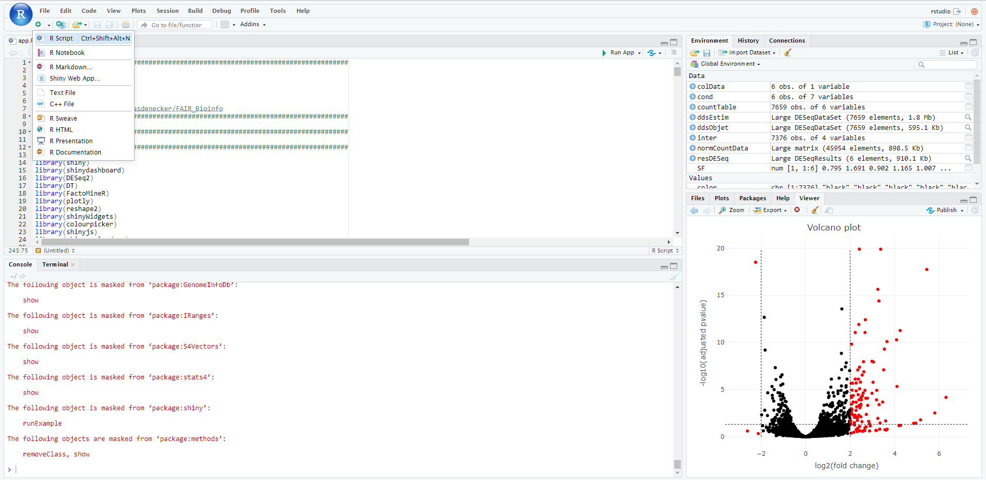
Exemple de base d'un Rnotebook
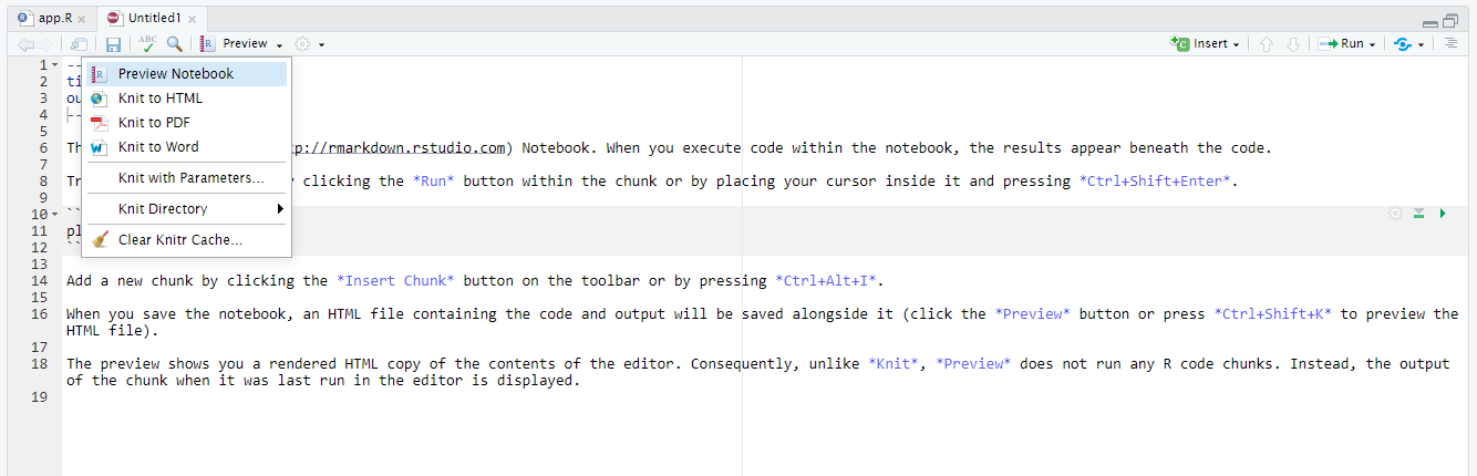
Enregistrer en html (ou PDF,...)
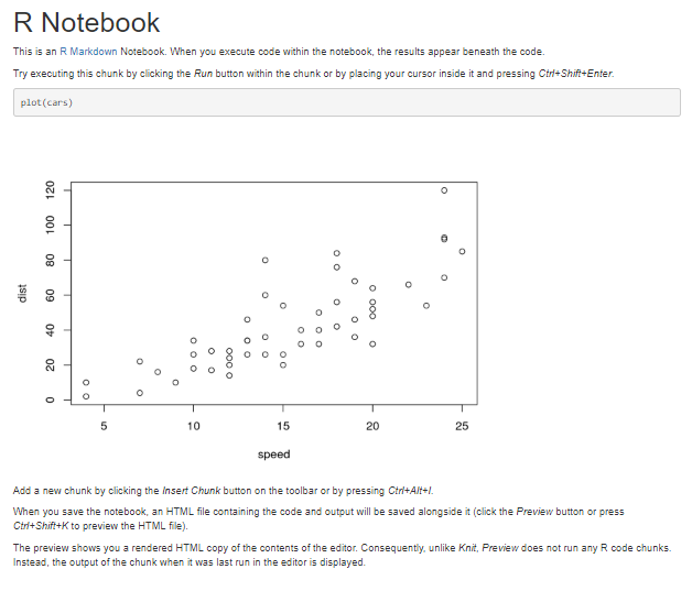
La page HTML obtenue
Construction d'un Rnotebook
Arguments du fichier (titre, type de sortie, arguments...)
---
title: "R Notebook"
output:
  html_document:
    df_print: paged
---
Du markdown (libre)
This is an [R Markdown](http://rmarkdown.rstudio.com) Notebook. When you execute code within the notebook, the results appear beneath the code.

Try executing this chunk by clicking the *Run* button within the chunk or by placing your cursor inside it and pressing *Ctrl+Shift+Enter*.
Du code (dans une zone)
```{r}
plot(cars)
```
Des arguments intéressants pour la zone de code
Le code n'est pas affiché
Une super ressource ! https://bookdown.org/yihui/rmarkdown/
```{r echo=FALSE}
plot(cars)
```
Le résultat n'est pas affiché
```{r results="hide"}
plot(cars)
```
Les alertes et messages ne sont pas affichés
```{r warning=FALSE, message=FALSE}
plot(cars)
```
+

Renforcement de la reproductibilité
Création automatique d'un rapport d'analyses avec Rmarkdown dans notre application Shiny
Pourquoi?
Avoir les figures et les résultats dans un fichier figé à une date et une heure données avec des arguments précis
Nous le combinerons avec un fichier qui enregistre les paramètres
Plan d'actions
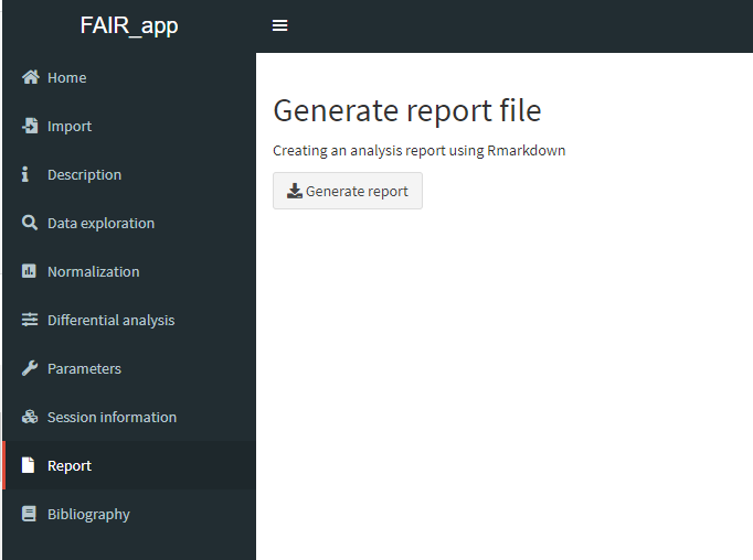
Un bouton pour générer un notebook (en HTML)
- Rapport d'analyse
- Fichier de paramètres
Mettre une zone de lecture pour les paramètres
- Lire le fichier
- Mettre à jour les paramètres
Le rapport (HTML)
Exemple disponible (Plotly)
Les codes
Code
app.R
report.Rmd

Paramètres
report.html
params.txt
Le bouton qui génère le fichier
Coté UI
downloadButton("reportBTN", "Generate report")Coté serveur
output$reportBTN <- downloadHandler(
filename = paste0("report_",data$date,".html"),
content = function(file) {
params <- list(si = si,
date = data$date,
dataCondition = data$conditions,
dataCountTable = data$countTable,
dataSummary = data$summary,
colorColConds = color$colConds,
deseqRV_resDESeq = deseqRV$resDESeq,
logFC= input$logFC,
pvalue= input$pvalue,
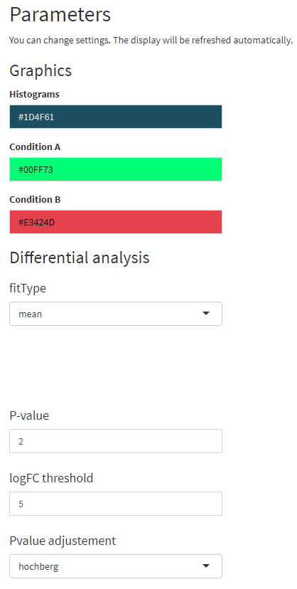
tableParams= c(ColHisto = input$colHisto,
ColCondA = input$colCondA,
ColCondB = input$colCondB,
fitType = input$fitType,
pvalue = input$pvalue,
logFC= input$logFC,
pAdjustMethod = input$pAdjustMethod))
rmarkdown::render("report.Rmd", output_file = file,
params = params,
envir = new.env(parent = globalenv())
)
}
)Le fichier Rmarkdown
---
title: "FAIR_Bioinfo analysis"
params:
dataCondition: NA
si: NA
colorColConds: NA
dataSummary: NA
dataCountTable : NA
deseqRV_resDESeq: NA
pvalue: NA
logFC: NA
tableParams: NA
date: NA
output:
html_document:
df_print: paged
---
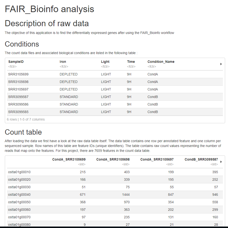
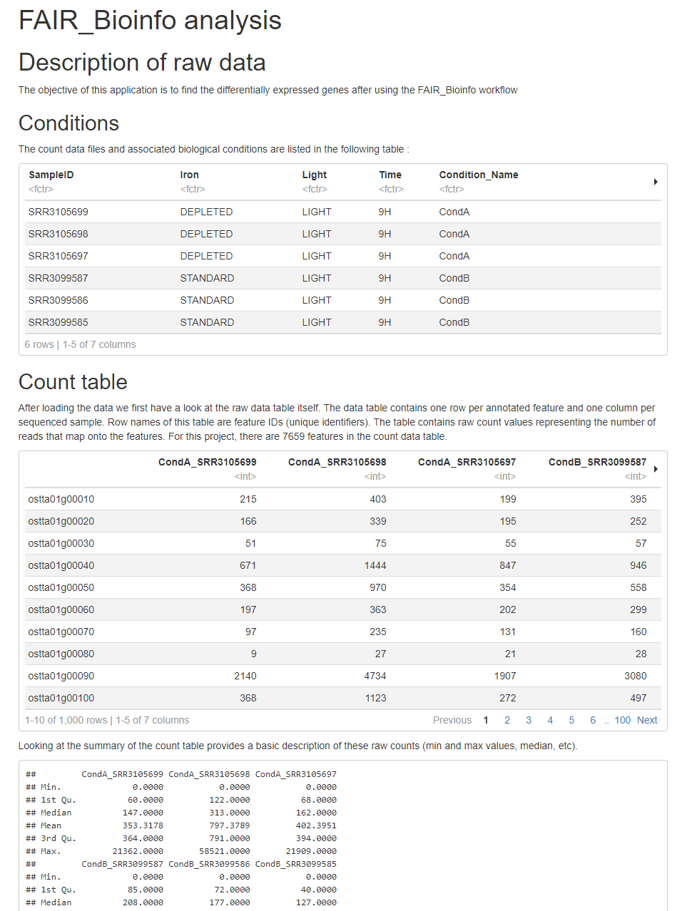
# Description of raw data
The objective of this application is to find the differentially expressed genes after using the FAIR_Bioinfo workflow
## Conditions
The count data files and associated biological conditions are listed in the following table :
```{r echo = F}
params$dataCondition
```
## Count table
After loading the data we first have a look at the raw data table itself. The data table contains one row per annotated feature and one column per sequenced sample. Row names of this table are feature IDs (unique identifiers). The table contains raw count values representing the number of reads that map onto the features. For this project, there are 7659 features in the count data table.
```{r echo = F}
params$dataCountTable
```
Looking at the summary of the count table provides a basic description of these raw counts (min and max values, median, etc).
```{r echo = F}
params$dataSummary
```
## Total read count per sample
Next figure shows the total number of mapped reads for each sample. Reads that map on multiple locations on the transcriptome are counted more than once, as far as they are mapped on less than 50 different loci. We expect total read counts to be similar within conditions, they may be different across conditions. Total counts sometimes vary widely between replicates. This may happen for several reasons, including:
- different rRNA contamination levels between samples (even between biological replicates);
- slight differences between library concentrations, since they may be difficult to measure with high precision.;
```{r echo = F}
barplot(colSums(params$dataCountTable), ylab = "Total read count per sample",
main = "Total read count", col = params$colorColConds,
names = colnames(params$dataCountTable))
```
[...]
## Volcano plot
```{r echo = F}
inter = cbind(x = params$deseqRV_resDESeq$log2FoldChange,
y = -log10(params$deseqRV_resDESeq$padj),
feature = rownames(params$deseqRV_resDESeq),
SE = params$deseqRV_resDESeq$lfcSE)
inter = na.omit(inter)
inter = as.data.frame(inter)
inter[,1] = as.numeric(as.character(inter[,1]))
inter[,2] = as.numeric(as.character(inter[,2]))
color = rep("black", nrow(inter))
pos = which(abs(inter$x) >= params$logFC & inter$y >= -log10(params$pvalue))
color[pos] = "red"
plot_ly(inter, x = ~x, y = ~y, type = 'scatter', mode = 'markers',
text = ~paste("Feature: ", feature, '<br>lfcSE:', SE),
marker = list(color = color)) %>%
layout(title = 'Volcano plot',
shapes=list(list(type='line', x0=min(inter$x)-1, x1= max(inter$x)+1, y0=-log10(params$pvalue), y1=-log10(params$pvalue), line=list(dash='dot', width=1)),
list(type='line', x0=-params$logFC, x1= -params$logFC, y0=0, y1=max(inter$y), line=list(dash='dot', width=1)),
list(type='line', x0=params$logFC, x1= params$logFC, y0=0, y1=max(inter$y), line=list(dash='dot', width=1))),
yaxis = list(zeroline = FALSE, title= "-log10(adjusted pvalue)"),
xaxis = list(zeroline = FALSE, title= "log2(fold change)"))
```
# Parameters
```{r echo = F}
params$tableParams
inter = cbind(names(params$tableParams),params$tableParams)
colnames(inter) = c("Params", "Values")
write.table( inter, paste0("params_",params$date,".txt"),
sep = "\t",
quote = F, row.names = F)
```
# R session information
The versions of the R software and Bioconductor packages used for this analysis are listed below. It is important to save them if one wants to re-perform the analysis in the same conditions.
```{r echo = F}
params$si
```Fichier de paramètres
Lors de la création du rapport, un fichier de paramètres est créé.
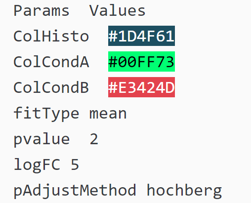
exampleFile_params.txt
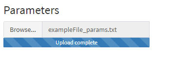

Import du fichier de paramètres
Côté UI
h3("Parameters"),
            fileInput("ParamsFile",label = NULL,
                      buttonLabel = "Browse...",
                      placeholder = "No file selected")
Côté serveur (après la lecture des données)
observeEvent(input$run, {

[...]

if(!is.null(input$ParamsFile$datapath)){
    data$Params <- read.csv2(input$ParamsFile$datapath,
                             header = T,
                             sep = "\t",
                             quote = ""
    )

    colourpicker::updateColourInput(session, "colHisto", value = data$Params[1,2])
    colourpicker::updateColourInput(session, "colCondA", value = data$Params[2,2])
    colourpicker::updateColourInput(session, "colCondB", value = data$Params[3,2])
    updateSelectInput(session, "fitType",  selected = data$Params[4,2])
    updateNumericInput(session, "pvalue", value = data$Params[5,2])
    updateNumericInput(session, "logFC", value = data$Params[6,2])
    updateSelectInput(session, "pAdjustMethod",  selected = data$Params[7,2])
}

[...]

})
Mise à jour des paramètres après import
Par défaut
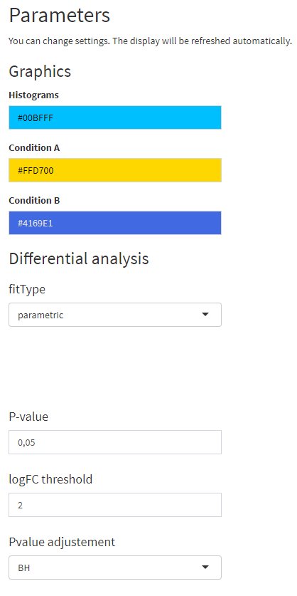
Après import du fichier exemple
Un exemple ?
Conclusion
Rmarkdown ou Jupyter ?
Idéal pour la génération d'un notebook automatique dans un projet R
Idéal pour tous les projets avec un aspect paramétrable par l'utilisateur
Autres langages que R
Bilan de la session
Création d'un rapport d'analyse
- Jupyter
- Rmarkdown
- Partage du notebook
- Augmentation de la reproductibilité de l'app FAIR_Bioinfo
- Rapport d'analyses
- Fichier de paramètres
Pour la prochaine fois
Ajouter dans l'application vue à la session précédente un bouton qui génère un Notebook contenant la figure et les paramètres graphiques

Bon courage !
RDV sur Slack en cas de problème